The Resurrection of the Computer Fridge

img_20190731_1837407130935668874283186.jpgThe computer fridge hypothesis is a seemingly brilliant idea: store and operate your computer in a fridge, and wave good bye to all heating issues.

However — in 2015, a disappointing video appeared on YouTube: Linus Tech Tips once and for all rejected the computer fridge hypothesis by an experiment showing that refrigerators always loose in thermodynamic battles against modern computers.

The heat dissipated by the personal computer will exceed the heat absorption capacity of the fridge evaporator — causing the ambient temperature in the fridge to rise rather than fall. If we consider the system as a whole, we have a serious self-heating problem, and there is nothing we can do about it.

Or is it?

Cracking The Self-Heating Problem

Pleasant ideas deserve to be treated with respect, right? They should be tried from every angle before being trashed. From first principles, I decided to challenge the rejection of the computer fridge hypothesis by proposing: the ventilated computer fridge hypothesis!

The Ventilated Computer Fridge Hypothesis

img_20190808_125029.jpg
A Ventilated Computer Fridge

The ventilated computer fridge hypothesis is based on the following reasoning: If the fridge is equipped with a balanced ventilation system, most of the heat dissipated by the computer will be transferred out of the fridge, so there will be no self-heating. When the fridge is turned off, the system will simply function as a normal computer cabinet. Now, if we in addition route the in-air stream via the evaporator, the air will be cold when it hits the computer, thus absorbing heat from the computer on the way out of the fridge. See the sketch on the right.

I decided to test the new hypothesis, so I had to build my own computer fridge.

Building a Computer Fridge

I bought a second hand mini-fridge with a glass door from TempTech on eBay as a starting point.

Installing Balanced Ventilation

bb138b1h3790128944658168010.jpgI decided to install a simple balanced ventilation system represented by four Corsair ML140 Pro cabinet fans.

While the task of installing four fans in a mini-fridge is not the most pleasant thing a human being can do in the world — it can be done by some laborious drilling on the outside, and heavy angle grinding on the inside.

My friend Øyvind Colliander created a nice template for the drilling part. See the fan hole template below. The trick is to tape a printed template to the fridge wall, and use a punch and a hammer to mark the center of the holes before drilling. For the angle grinding, put on a face mask and cut out four squares on the inside aligned with the holes on the outside.

Result: two fans on the upper back (in-air), and one fan on each side (out-air).

IMG_20190806_100327
Fan holes on the sides
IMG_20190806_100311
Fan holes on the back
holepattern
Fan hole template for Corsair ML140 Pro (A4 print-friendly PDF)

Bypassing the Thermostat & More

In order to get full control of the fridge’s cooling system, I bypassed the internal thermostat and instead installed an Arduino micro controller and an external relay board beneath the back plate on the inside of the fridge. I also permanently installed the Arduino DHT-11 sensor to get ambient temperature and humidity readings. The sensor is placed in the bottom right corner of the fridge. I drilled holes on the backside for 230 VAC power and Ethernet, and installed a power socket, as well as two AC/DC converters (36 VDC & 12 VDC) on the inside.

Lighting and a Retractable Shelf

At this point, the fridge was ready to be tested, but for fun I decided to take the concept just a few steps further… Some lighting is nice, right? And — uh, a motorized retractable shelf for the computer! The latter turned out to be more challenging.

Basically, I used FreeCad to design a rack-and-pinion based retractable shelf. The design consists of three main parts; the rack, an old electric parabola antenna motor with a pinion, and a clamp to fix it to the shelf. Thanks to Andre Böehme for helping out with the toughest part — namely modelling the pinion and a matching rack tooth profile. I used i.materialise to 3D-print the parts. Great service!

test
Retractable Shelf Design

ejectTo control the position and direction of retraction of the shelf, I combined two of the relays on the external relay board to achieve a polarity reversal switch.

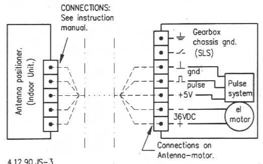
The parabola antenna motor also has a built-in pulse counter circuit, which can be used to pinpoint its exact angular position. Basically, the circuit sends out short square pulses synchronized with the pinions angular movement. Position control is thus achieved by simply counting pulses with an analog input channel on the Arduino.

See below for a full (sloppy) wiring diagram of the system.

IMG_20190807_103728

Installing the Computer

img_20190731_1837407130935668874283186.jpg

I installed the computer hardware on a Lian Li test bench placed on top of the retractable shelf in the fridge.

Computer Specifications: 

  • ASUS ROG STRIX B450-E GAMING Motherboard
  • AMD Ryzen 5 2600 Wraith Stealth
  • Corsair Vengeance LPX DDR4-3200 C16 BK DC – 32GB
  • Samsung 970 EVO Plus SSD M.2 2280 – 500GB
  • ASUS GeForce RTX 2080 Ti ROG STRIX OC – 11GB GDDR6 RAM
  • Corsair 1000W PSU

Computer Fridge Code

The software I developed for the computer fridge basically consists of three parts;

  • An embedded Arduino back-end coded in C (deepfridge.ino)
  • A Python CLI frond-end to control the whole system (deepfridge.py)
Screenshot from 2019-08-09 11-47-03.png
Deep Fridge CLI
  • A set of Python test scripts with data logging functionality to conduct experiments (tests/deepfridge_logger_test*.py)

The code is available on Github: https://github.com/gknilsen/computer_fridge

The Computer Fridge Put at Test

Let’s run a series of tests to see if the computer fridge works. We will use the test scripts tests/deepfridge_logger_test*.py included in the Github repository. The test scripts log the following parameters to CSV files;

  • Fridge temperature  (by deepfridge.ino / Arduino DHT-11 sensor)
  • Fridge humidity (by deepfridge.ino / Arduino DHT-11 sensor)
  • CPU temperature (by calls to lmsensors / integrated CPU thermistor)
  • CPU utilization (by calls to cpu_usage.sh which is based on calls to top)
  • GPU temperature (by calls to nvidia-smi / integrated GPU thermistor)
  • GPU utilization (by calls to nvidia-smi)

Some of the tests put the CPU and/or GPU to maximum utilization under certain periods — this is achieved by calls to stress and gpu-burn.

Test #1 — Computer CPU & GPU at Idle with Cooling

Description: The computer CPU & GPU is left at idle. First run for 5 minutes when the compressor is OFF to get a baseline, then the compressor is turned ON, and the logging continues for 55 minutes. Total test time is 1 hour (3600 seconds).

Test script: tests/deepfridge_logger_test1.py

Log file: tests/test1.csv

Result:

Test_1

Conclusion: Running the compressor for about an hour results in a CPU & GPU temperature drop of 5 degrees Celsius, when the computer is at idle. Also the ambient fridge temperature is reduced by 5 degrees Celsius.

Test #2 — Computer CPU at Maximum Utilization without Cooling

Description: The computer CPU is left at idle the first 5 minutes, and the compressor is OFF, to get a baseline. Then the computer CPU is put on maximum utilization for 5 minutes. The computer CPU is then left at idle for 5 minutes more minutes. Total test time is 15 minutes (900 seconds).

Test script: deepfridge_logger_test2.py

Log file: tests/test2.csv

Result:

Test_2

Conclusion: Peak CPU temperature under max utilization is at 53.7 degrees Celsius.

Test #3 — Computer CPU at Maximum Utilization with Cooling

Description: The compressor is set ON, and the computer is left at idle the first 45 minutes. Then the computer CPU is put at maximum load for 5 minutes, followed by 10 more minutes at idle. Total test time is 60 minutes (3600 seconds).

Test script: deepfridge_logger_test3.py

Log file: tests/test3.csv

Result:

Test_3

Conclusion: With constant cooling for about one hour & max CPU utilization for 5 minutes, again the CPU temperature is reduced by 5 degrees Celsius. Also the ambient fridge temperature is reduced by 5 degrees Celsius.

Test #4 — Computer GPU at Maximum Utilization without Cooling

Description: The computer GPU is left at idle the first 5 minutes, and the compressor is OFF, to get a baseline. Then the computer GPU is put at maximum utilization for 5 minutes. The computer GPU is then left at idle for 5 minutes more minutes. Total test time is 15 minutes (900 seconds).

Test script: deepfridge_logger_test4.py

Resulting log file: test4.csv

Result:

Test_4

Conclusion: Peak GPU temperature under max utilization is at 66 degrees Celsius.

Test #5 — Computer GPU at Maximum Utilization with Cooling

Description: The compressor is set ON, and the computer is left at idle the first 45 minutes. Then the computer GPU is put on maximum load for 5 minutes, followed by 10 more minutes at idle. Total test time is 60 minutes (3600 seconds).

Test script: deepfridge_logger_test5.py

Log file: tests/test5.csv

Result:

Test_5

Conclusion: With constant cooling for about one hour & max GPU utilization for 5 minutes, the GPU temperature is reduced by 3 degrees Celsius. The ambient fridge temperature is reduced by 4 degrees Celsius.

Conclusion

The tests show that there are no signs of self-heating, and that the CPU/GPU temperature drops 3-5 degrees Celsius when the cooling system has been activated for about an hour.

The ventilated computer fridge hypothesis has been confirmed!

However, is a temperature drop of 3-5 degrees Celsius worth the effort? Well, it depends. If you play around with overclocking and want to squeeze the most out of your system, 3-5 degrees Celsius might be enough. But is it really worth the effort? The system complexity is overwhelming, costly and not especially effective in its current state. However, the project was a great learning experience, and it was really fun! I doubt that I will run the cooling system much in its current state on a daily basis though.

There is plenty of room for optimization. In fact, currently I have not tested to see what happens if the cooling system remains activated for a longer period than one hour. Same is true for extended periods of maximum CPU/GPU utilization.

Please leave your thoughts in the comments section below. I am happy to receive ideas which can potentially improve the cooling performance of the system.

Coding a Parametric Equalizer for Audio Applications

As a kid I was very fascinated by a particular type of electronic devices known as equalizers. These devices are used to adjust the balance between frequency components of electronic signals, and has a widespread application in audio engineering.

As I grew up the fascination continued, but shifted from wanting to own one — into wanting to build one — into wanting to code one.

eqpic.jpg
Image credit: http://www.lifewire.com

Introduction

In this article I will explain how you can code your own audio equalizer, enabling you to integrate your own variant in your own projects. Let us start with some background information and basic theory.

When you use the volume knob to pump up the volume on your stereo, it will boost all the frequency components of the audio by roughly the same amount. The bass and treble controls on some stereos take this concept one step further; they divide the whole frequency range into two parts — where the bass knob controls the volume in the lower frequency range and the treble knob controls the volume in the upper frequency range.

Now, with an audio equalizer, you have the possibility to adjust the volume on any given number of  individual frequency ranges, separately.

Physically, the front panel of an equalizer device typically consists of a collection of slider knobs, each corresponding to a given frequency range — or more specifically — to a given center frequency. The term center frequency refers to the mid point of the frequency range the slider knob controls.

By arranging the sliders in increasing center frequency order, the combined positions of the individual sliders will represent the overall frequency response of the equalizer. This is where it gets interesting, because the horizontal position of the slider now represents frequency, and the vertical position represents the response modification you wish to impose on that frequency. In other words, you can “draw” your desired frequency response by arranging the sliders accordingly.

Theory of Parametric Equalizers

An additional degree of freedom arises when the center frequency per slider also is adjustable. This is exactly what a parametric equalizer is: it lets the user specify a number of sections (think of section here as a slider), each with a frequency response adjustable by the following parameters: center frequency (f0), bandwidth (Bf), bandwidth gain (GB), reference gain (G0) and boost/cut gain (G):

  • The center frequency (f0) represents the mid-point of the section’s frequency range and is given in Hertz [Hz].
  • The bandwidth (Bf) represents the width of the section across frequency and is measured in Hertz [Hz]. A low bandwidth corresponds to a narrow frequency range meaning that the section will concentrate its operation to only the frequencies close to the center frequency. On the other hand, a high bandwidth yields a section of wide frequency range — affecting a broader range of frequencies surrounding the center frequency.
  • The bandwidth gain (GB) is given in decibels [dB] and represents the level at which the bandwidth is measured. That is, to have a meaningful measure of bandwidth, we must define the level at which it is measured. See Figure 1.
  • The reference gain (G0) is given in decibels [dB] and simply represents the level of the section’s offset. See Figure 1.
  • The boost/cut gain (G) is given in decibels [dB] and prescribes the effect imposed on the audio loudness for the section’s frequency range. A boost/cut level of 0 dB corresponds to unity (no operation), whereas negative numbers corresponds to cut (volume down) and positive numbers to boost (volume up).
section.png
Figure 1: Section Frequency Spectrum

A section is really just a filter — in our case a digital audio filter with the parameters corresponding to the elements in the list above.

Implementation in Matlab

The abstraction now is the following: a parametric audio equalizer is nothing else than a list of digital audio filters acting on the input signal to produce an output signal with the desired balance between frequency components.

This means that the smallest building block we need to create is a digital audio filter. Without going deep into the field of digital filter design, I will make it easy for you and jump straight to the crucial equation required:

Equation 1

a0*y(n) = b0*x(n) + b1*x(n-1) + b2*x(n-2)
        - a1*y(n-1) - a2*y(n-2), for n = 0, 1, 2, ...

In equation 1, x(n) represents the input signal, y(n) the output signal, a0, a1 and a2, are the feedback filter coefficients, and b0, b1 and b2, are the feedforward filter coefficients.

To calculate the filtered output signal, y(n), all you have to do is to run the input signal, x(n), through the recurrence relation given by equation 1. In Matlab, equation 1 corresponds to the filter function. We will come back to it shortly, but first we need to get hold of the filter coefficients (a0, a1, a2, b0, b1 and b2).

At this point, you can read Orfanidis’ paper and try to grasp the underlying mathematics, but I will make it easy for you. Firstly, we define the sampling rate of the input signal x(n) as fs, and secondly, by using the section parameters defined above, the corresponding filter coefficients can be calculated by

Equations 2 – 8

beta = tan(Bf/2*pi/(fs/2))*sqrt(abs((10^(GB/20))^2
     - (10^(G0/20))^2))/sqrt(abs(10^(G/20)^2 - (10^(GB/20))^2))

b0 = (10^(G0/20) + 10^(G/20)*beta)/(1+beta)
b1 = -2*10^(G0/20)*cos(f0*pi/(fs/2))/(1+beta) 
b2 = (10^(G0/20) - 10^(G/20)*beta)/(1+beta)

a0 = 1
a1 = -2*cos(f0*pi/(fs/2))/(1+beta)
a2 = (1-beta)/(1+beta)

Note that beta in equation 2 is just used as an intermediate variable to simplify the appearance of equations 3 through 8. Also note that tan() and cos() represents the tangens and cosine functions, respectively, pi represents 3.1415…, and sqrt() is the square root.

As an example, if we define the following section parameters:

(fs, f0, Bf, GB, G0, G) = (1000, 250, 40, 9, 0, 12)

It means that we will have a section operating at a 1 kHz sampling rate with a center frequency of 250 Hz, bandwidth of 40 Hz, bandwidth gain of 9 dB, reference gain of 0 dB and boost gain of 12 dB. See Figure 2 for the frequency response (spectrum) of the section.

section_ex
Figure 2: Example Section Frequency Spectrum

Let’s say we have defined a list of many sections. How do we combine all the sections together so we can see the overall result? The following Matlab script illustrates the concept by setting up a 4-section parametric equalizer.

% Parametric Equalizer by Geir K. Nilsen (2017)
clear all;

fs = 1000; % Sampling frequency [Hz]
S = 4; % Number of sections

Bf = [5 5 5 5]; % Bandwidth [Hz]
GB = [9 9 9 9]; % Bandwidth gain (level at which the bandwidth is measured) [dB]
G0 = [0 0 0 0]; % Reference gain @ DC [dB]
G = [8 10 12 14]; % Boost/cut gain [dB]
f0 = [200 250 300 350]; % Center freqency [Hz]

h = [1; zeros(1023,1)]; % ..for impulse response
b = zeros(S,3); % ..for feedforward filter coefficients
a = zeros(S,3); % ..for feedbackward filter coefficients

for s = 1:S;
    % Equation 2
    beta = tan(Bf(s)/2 * pi / (fs / 2)) * sqrt(abs((10^(GB(s)/20))^2 - (10^(G0(s)/20))^2)) / sqrt(abs(10^(G(s)/20)^2 - (10^(GB(s)/20))^2));
    % Equation 3 through 5
    b(s,:) = [(10^(G0(s)/20) + 10^(G(s)/20)*beta), -2*10^(G0(s)/20)*cos(f0(s)*pi/(fs/2)), (10^(G0(s)/20) - 10^(G(s)/20)*beta)] / (1+beta);
    % Equation 6 through 8
    a(s,:) = [1, -2*cos(f0(s)*pi/(fs/2))/(1+beta), (1-beta)/(1+beta)];

    % apply equation 1 recursively per section.
    h = filter(b(s,:), a(s,:), h);
end;

% Plot the frequency spectrum of the combined section impulse response h
H = db(abs(fft(h)));
H = H(1:length(H)/2);
f = (0:length(H)-1)/length(H)*fs/2;
plot(f,H)
axis([0 fs/2 0 20])
xlabel('Frequency [Hz]');
ylabel('Gain [dB]');
grid on

The key to combining the sections is to run the input signal through the sections in a cascaded fashion: the output signal of the first section is fed as input to the next section, and so on. In the script above, the input signal is set to the delta function, so that the output of the first section yields its impulse response — which in turn is fed as the input to the next section, and so on. The final output of the last section is therefore the combined (total) impulse response of all the sections, i.e. the impulse response of the parametric equalizer.

The FFT is then applied on the overall impulse response to calculate the frequency response, which finally is used to produce the frequency spectrum of the equalizer shown in Figure 3.

eq response
Figure 3: Parametric Equalizer Frequency Spectrum

The next section of this article will address how to make the step from the Matlab implementation above to a practical implementation in C#. Specifically, I will address:

  • How to run the equalizer in real-time, i.e. how to apply it in a system where only few samples of the actual input signal is available at the same time — and furthermore ensure that the combined output signals will be continuous (no hiccups).
  • How to object orientate the needed parts of the implementation.

Real-time considerations

Consider equation 1 by evaluating it for n=0,1,2, and you will notice that some of the  indices on the right hand side of the equation will be negative. These terms with negative index correspond to the recurrence relation’s initial conditions. If we consider the recurrence relation as a one-go operation, it is safe to set those terms to zero. But what if we have a real system sampling a microphone at a rate of fs=1000 Hz, and where the input signal x(n) is made available in a finite length buffer of size 1000 samples — updated by the system once every second?

To ensure that the combined output signals will be continuous, the initial conditions must be set based on the previous states of the recurrence relation. In other words, the recurrence relation implementation must have some memory of its previous states. Specifically, it means that at the end of the function implementing the recurrence relation, one must store the two last samples of the current output and input signals. When the next iteration starts, it will use those values as the initial conditions y(-1), y(-2), x(-1) and x(-2).

A practical C# Implementation

I will now give a practical implementation in C#. It consists of three classes

  • Filter.cs — Implements the recurrence relation given in equation 1. And yes, it is made to deal gracefully with the initial condition problem stated in the previous section.
  • Section.cs — Implements a section as described by the parameters listed previously.
  • ParametricEqualizer.cs — Implements the parametric equalizer.

Filter.cs

/* @author Geir K. Nilsen (geir.kjetil.nilsen@gmail.com) 2017 */

namespace ParametricEqualizer
{
    public class Filter
    {
        private List a;
        private List b;

        private List x_past;
        private List y_past;

        public Filter(List a, List b)
        {
            this.a = a;
            this.b = b;
        }

        public void apply(List x, out List y)
        {
            int ord = a.Count - 1;
            int np = x.Count - 1;

            if (np < ord)
            {
                for (int k = 0; k < ord - np; k++)
                    x.Add(0.0);
                np = ord;
            }

            y = new List();
            for (int k = 0; k < np + 1; k++)
            {
                y.Add(0.0);
            }

            if (x_past == null)
            {
                x_past = new List();

                for (int s = 0; s < x.Count; s++)
                    x_past.Add(0);
            }

            if (y_past == null)
            {
                y_past = new List();

                for (int s = 0; s < y.Count; s++)
                    y_past.Add(0);
            }

            for (int i = 0; i < np + 1; i++)
            {
                y[i] = 0.0;

                for (int j = 0; j < ord + 1; j++)
                {
                    if (i - j < 0)
                        y[i] = y[i] + b[j] * x_past[x_past.Count - j];
                    else
                        y[i] = y[i] + b[j] * x[i - j];
                }

                for (int j = 0; j < ord; j++)
                {
                    if (i - j - 1 < 0)
                        y[i] = y[i] - a[j + 1] * y_past[y_past.Count - j - 1];
                    else
                        y[i] = y[i] - a[j + 1] * y[i - j - 1];
                }

                y[i] = y[i] / a[0];
            }

            x_past = x;
            y_past = y;

        }
    }
}

Section.cs

/* @author Geir K. Nilsen (geir.kjetil.nilsen@gmail.com) 2017 */

namespace ParametricEqualizer
{
    public class Section
    {
        private Filter filter;
        private double G0;
        private double G;
        private double GB;
        private double f0;
        private double Bf;
        private double fs;

        private double[][] coeffs;

        public Section(double f0, double Bf, double GB, double G0, double G, double fs)
        {
            this.f0 = f0;
            this.Bf = Bf;
            this.GB = GB;
            this.G0 = G0;
            this.G = G;
            this.fs = fs;

            this.coeffs = new double[2][];
            this.coeffs[0] = new double[3];
            this.coeffs[1] = new double[3];

            double beta = Math.Tan(Bf / 2.0 * Math.PI / (fs / 2.0)) * Math.Sqrt(Math.Abs(Math.Pow(Math.Pow(10, GB / 20.0), 2.0) - Math.Pow(Math.Pow(10.0, G0 / 20.0), 2.0))) / Math.Sqrt(Math.Abs(Math.Pow(Math.Pow(10.0, G / 20.0), 2.0) - Math.Pow(Math.Pow(10.0, GB/20.0), 2.0)));

            coeffs[0][0] = (Math.Pow(10.0, G0 / 20.0) + Math.Pow(10.0, G/20.0) * beta) / (1 + beta);
            coeffs[0][1] = (-2 * Math.Pow(10.0, G0/20.0) * Math.Cos(f0 * Math.PI / (fs / 2.0))) / (1 + beta);
            coeffs[0][2] = (Math.Pow(10.0, G0/20) - Math.Pow(10.0, G/20.0) * beta) / (1 + beta);

            coeffs[1][0] = 1.0;
            coeffs[1][1] = -2 * Math.Cos(f0 * Math.PI / (fs / 2.0)) / (1 + beta);
            coeffs[1][2] = (1 - beta) / (1 + beta);

            filter = new Filter(coeffs[1].ToList(), coeffs[0].ToList());
        }

        public List run(List x, out List y)
        {
            filter.apply(x, out y);
            return y;
        }
    }
}

ParametricEqualizer.cs

namespace ParametricEqualizer
{
    public class ParametricEqualizer
    {
        private int numberOfSections;
        private List section; 
        private double[] G0; 
        private double[] G; 
        private double[] GB; 
        private double[] f0; 
        private double[] Bf; 

        public ParametricEqualizer(int numberOfSections, int fs, double[] f0, double[] Bf, double[] GB, double[] G0, double[] G) 
        { 
            this.numberOfSections = numberOfSections; 
            this.G0 = G0; 
            this.G = G; 
            this.GB = GB; 
            this.f0 = f0; 
            this.Bf = Bf; 
            section = new List();
            for (int sectionNumber = 0; sectionNumber < numberOfSections; sectionNumber++) 
            { 
                section.Add(new Section(f0[sectionNumber], Bf[sectionNumber], GB[sectionNumber], G0[sectionNumber], G[sectionNumber], fs));
            } 
        } 
         
        public void run(List x, ref List y) 
        { 
            for (int sectionNumber = 0; sectionNumber < numberOfSections; sectionNumber++) 
            { 
                section[sectionNumber].run(x, out y); 
                x = y; // next section 
            } 
        } 
    }
}

Usage Example

Let’s conclude the article by an example where we create a ParamtricEqualizer object and applies it on some input data. The following snippet will setup the equivalent 4-section equalizer as in the Matlab implementation above.

double[] x = new double[] { 1.0, 0.0, 0.0, 0.0, 0.0, 0.0, 0.0, 0.0, 0.0, 0.0}; // input signal (delta function example)
List y = new List(); // output signal
ParametricEqualizer.ParametricEqualizer peq = new ParametricEqualizer.ParametricEqualizer(4, 1000, new double[] { 200, 250, 300, 350 }, new double[] { 5, 5, 5, 5 }, new double[] { 9, 9, 9, 9 }, new double[] {0, 0, 0, 0}, new double[] {8, 10, 12, 14});
peq.run(x.ToList(), ref y);