Author: gknilsen

As a kid I was very fascinated by a particular type of electronic devices known as equalizers. These devices are used to adjust the balance between frequency components of electronic signals, and has a widespread application in audio engineering.

As I grew up the fascination continued, but shifted from wanting to own one — into wanting to build one — into wanting to code one.

Introduction

In this article I will explain how you can code your own audio equalizer, enabling you to integrate your own variant in your own projects. Let us start with some background information and basic theory.

When you use the volume knob to pump up the volume on your stereo, it will boost all the frequency components of the audio by roughly the same amount. The bass and treble controls on some stereos take this concept one step further; they divide the whole frequency range into two parts — where the bass knob controls the volume in the lower frequency range and the treble knob controls the volume in the upper frequency range.

Now, with an audio equalizer, you have the possibility to adjust the volume on any given number of  individual frequency ranges, separately.

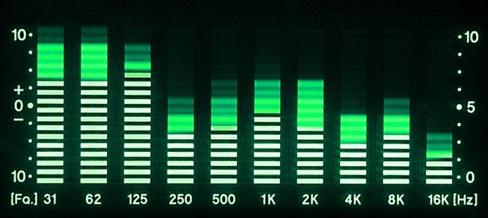
Physically, the front panel of an equalizer device typically consists of a collection of slider knobs, each corresponding to a given frequency range — or more specifically — to a given center frequency. The term center frequency refers to the mid point of the frequency range the slider knob controls.

By arranging the sliders in increasing center frequency order, the combined positions of the individual sliders will represent the overall frequency response of the equalizer. This is where it gets interesting, because the horizontal position of the slider now represents frequency, and the vertical position represents the response modification you wish to impose on that frequency. In other words, you can “draw” your desired frequency response by arranging the sliders accordingly.

Theory of Parametric Equalizers

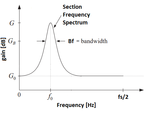
An additional degree of freedom arises when the center frequency per slider also is adjustable. This is exactly what a parametric equalizer is: it lets the user specify a number of sections (think of section here as a slider), each with a frequency response adjustable by the following parameters: center frequency (f0), bandwidth (Bf), bandwidth gain (GB), reference gain (G0) and boost/cut gain (G):

• The center frequency (f0) represents the mid-point of the section’s frequency range and is given in Hertz [Hz].
• The bandwidth (Bf) represents the width of the section across frequency and is measured in Hertz [Hz]. A low bandwidth corresponds to a narrow frequency range meaning that the section will concentrate its operation to only the frequencies close to the center frequency. On the other hand, a high bandwidth yields a section of wide frequency range — affecting a broader range of frequencies surrounding the center frequency.
• The bandwidth gain (GB) is given in decibels [dB] and represents the level at which the bandwidth is measured. That is, to have a meaningful measure of bandwidth, we must define the level at which it is measured. See Figure 1.
• The reference gain (G0) is given in decibels [dB] and simply represents the level of the section’s offset. See Figure 1.
• The boost/cut gain (G) is given in decibels [dB] and prescribes the effect imposed on the audio loudness for the section’s frequency range. A boost/cut level of 0 dB corresponds to unity (no operation), whereas negative numbers corresponds to cut (volume down) and positive numbers to boost (volume up).

A section is really just a filter — in our case a digital audio filter with the parameters corresponding to the elements in the list above.

Implementation in Matlab

The abstraction now is the following: a parametric audio equalizer is nothing else than a list of digital audio filters acting on the input signal to produce an output signal with the desired balance between frequency components.

This means that the smallest building block we need to create is a digital audio filter. Without going deep into the field of digital filter design, I will make it easy for you and jump straight to the crucial equation required:

Equation 1

a0*y(n) = b0*x(n) + b1*x(n-1) + b2*x(n-2)
        - a1*y(n-1) - a2*y(n-2), for n = 0, 1, 2, ...

In equation 1, x(n) represents the input signal, y(n) the output signal, a0, a1 and a2, are the feedback filter coefficients, and b0, b1 and b2, are the feedforward filter coefficients.

To calculate the filtered output signal, y(n), all you have to do is to run the input signal, x(n), through the recurrence relation given by equation 1. In Matlab, equation 1 corresponds to the filter function. We will come back to it shortly, but first we need to get hold of the filter coefficients (a0, a1, a2, b0, b1 and b2).

At this point, you can read Orfanidis’ paper and try to grasp the underlying mathematics, but I will make it easy for you. Firstly, we define the sampling rate of the input signal x(n) as fs, and secondly, by using the section parameters defined above, the corresponding filter coefficients can be calculated by

Equations 2 – 8

beta = tan(Bf/2*pi/(fs/2))*sqrt(abs((10^(GB/20))^2
     - (10^(G0/20))^2))/sqrt(abs(10^(G/20)^2 - (10^(GB/20))^2))

b0 = (10^(G0/20) + 10^(G/20)*beta)/(1+beta)
b1 = -2*10^(G0/20)*cos(f0*pi/(fs/2))/(1+beta) 
b2 = (10^(G0/20) - 10^(G/20)*beta)/(1+beta)

a0 = 1
a1 = -2*cos(f0*pi/(fs/2))/(1+beta)
a2 = (1-beta)/(1+beta)

Note that beta in equation 2 is just used as an intermediate variable to simplify the appearance of equations 3 through 8. Also note that tan() and cos() represents the tangens and cosine functions, respectively, pi represents 3.1415…, and sqrt() is the square root.

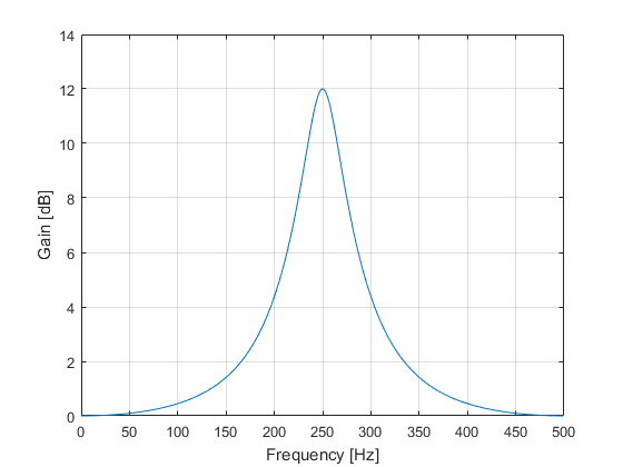
As an example, if we define the following section parameters:

(fs, f0, Bf, GB, G0, G) = (1000, 250, 40, 9, 0, 12)

It means that we will have a section operating at a 1 kHz sampling rate with a center frequency of 250 Hz, bandwidth of 40 Hz, bandwidth gain of 9 dB, reference gain of 0 dB and boost gain of 12 dB. See Figure 2 for the frequency response (spectrum) of the section.

Let’s say we have defined a list of many sections. How do we combine all the sections together so we can see the overall result? The following Matlab script illustrates the concept by setting up a 4-section parametric equalizer.

% Parametric Equalizer by Geir K. Nilsen (2017)
clear all;

fs = 1000; % Sampling frequency [Hz]
S = 4; % Number of sections

Bf = [5 5 5 5]; % Bandwidth [Hz]
GB = [9 9 9 9]; % Bandwidth gain (level at which the bandwidth is measured) [dB]
G0 = [0 0 0 0]; % Reference gain @ DC [dB]
G = [8 10 12 14]; % Boost/cut gain [dB]
f0 = [200 250 300 350]; % Center freqency [Hz]

h = [1; zeros(1023,1)]; % ..for impulse response
b = zeros(S,3); % ..for feedforward filter coefficients
a = zeros(S,3); % ..for feedbackward filter coefficients

for s = 1:S;
    % Equation 2
    beta = tan(Bf(s)/2 * pi / (fs / 2)) * sqrt(abs((10^(GB(s)/20))^2 - (10^(G0(s)/20))^2)) / sqrt(abs(10^(G(s)/20)^2 - (10^(GB(s)/20))^2));
    % Equation 3 through 5
    b(s,:) = [(10^(G0(s)/20) + 10^(G(s)/20)*beta), -2*10^(G0(s)/20)*cos(f0(s)*pi/(fs/2)), (10^(G0(s)/20) - 10^(G(s)/20)*beta)] / (1+beta);
    % Equation 6 through 8
    a(s,:) = [1, -2*cos(f0(s)*pi/(fs/2))/(1+beta), (1-beta)/(1+beta)];

    % apply equation 1 recursively per section.
    h = filter(b(s,:), a(s,:), h);
end;

% Plot the frequency spectrum of the combined section impulse response h
H = db(abs(fft(h)));
H = H(1:length(H)/2);
f = (0:length(H)-1)/length(H)*fs/2;
plot(f,H)
axis([0 fs/2 0 20])
xlabel('Frequency [Hz]');
ylabel('Gain [dB]');
grid on

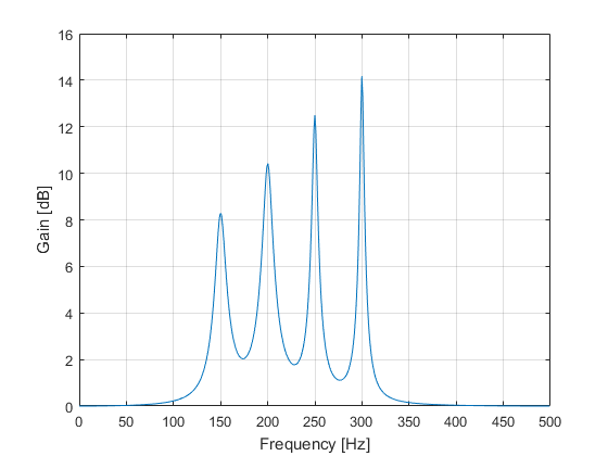
The key to combining the sections is to run the input signal through the sections in a cascaded fashion: the output signal of the first section is fed as input to the next section, and so on. In the script above, the input signal is set to the delta function, so that the output of the first section yields its impulse response — which in turn is fed as the input to the next section, and so on. The final output of the last section is therefore the combined (total) impulse response of all the sections, i.e. the impulse response of the parametric equalizer.

The FFT is then applied on the overall impulse response to calculate the frequency response, which finally is used to produce the frequency spectrum of the equalizer shown in Figure 3.

The next section of this article will address how to make the step from the Matlab implementation above to a practical implementation in C#. Specifically, I will address:

• How to run the equalizer in real-time, i.e. how to apply it in a system where only few samples of the actual input signal is available at the same time — and furthermore ensure that the combined output signals will be continuous (no hiccups).

• How to object orientate the needed parts of the implementation.

Real-time considerations

Consider equation 1 by evaluating it for n=0,1,2, and you will notice that some of the  indices on the right hand side of the equation will be negative. These terms with negative index correspond to the recurrence relation’s initial conditions. If we consider the recurrence relation as a one-go operation, it is safe to set those terms to zero. But what if we have a real system sampling a microphone at a rate of fs=1000 Hz, and where the input signal x(n) is made available in a finite length buffer of size 1000 samples — updated by the system once every second?

To ensure that the combined output signals will be continuous, the initial conditions must be set based on the previous states of the recurrence relation. In other words, the recurrence relation implementation must have some memory of its previous states. Specifically, it means that at the end of the function implementing the recurrence relation, one must store the two last samples of the current output and input signals. When the next iteration starts, it will use those values as the initial conditions y(-1), y(-2), x(-1) and x(-2).

A practical C# Implementation

I will now give a practical implementation in C#. It consists of three classes

• Filter.cs — Implements the recurrence relation given in equation 1. And yes, it is made to deal gracefully with the initial condition problem stated in the previous section.
• Section.cs — Implements a section as described by the parameters listed previously.
• ParametricEqualizer.cs — Implements the parametric equalizer.

Filter.cs

/* @author Geir K. Nilsen (geir.kjetil.nilsen@gmail.com) 2017 */

namespace ParametricEqualizer
{
    public class Filter
    {
        private List a;
        private List b;

        private List x_past;
        private List y_past;

        public Filter(List a, List b)
        {
            this.a = a;
            this.b = b;
        }

        public void apply(List x, out List y)
        {
            int ord = a.Count - 1;
            int np = x.Count - 1;

            if (np < ord)
            {
                for (int k = 0; k < ord - np; k++)
                    x.Add(0.0);
                np = ord;
            }

            y = new List();
            for (int k = 0; k < np + 1; k++)
            {
                y.Add(0.0);
            }

            if (x_past == null)
            {
                x_past = new List();

                for (int s = 0; s < x.Count; s++)
                    x_past.Add(0);
            }

            if (y_past == null)
            {
                y_past = new List();

                for (int s = 0; s < y.Count; s++)
                    y_past.Add(0);
            }

            for (int i = 0; i < np + 1; i++)
            {
                y[i] = 0.0;

                for (int j = 0; j < ord + 1; j++)
                {
                    if (i - j < 0)
                        y[i] = y[i] + b[j] * x_past[x_past.Count - j];
                    else
                        y[i] = y[i] + b[j] * x[i - j];
                }

                for (int j = 0; j < ord; j++)
                {
                    if (i - j - 1 < 0)
                        y[i] = y[i] - a[j + 1] * y_past[y_past.Count - j - 1];
                    else
                        y[i] = y[i] - a[j + 1] * y[i - j - 1];
                }

                y[i] = y[i] / a[0];
            }

            x_past = x;
            y_past = y;

        }
    }
}

Section.cs

/* @author Geir K. Nilsen (geir.kjetil.nilsen@gmail.com) 2017 */

namespace ParametricEqualizer
{
    public class Section
    {
        private Filter filter;
        private double G0;
        private double G;
        private double GB;
        private double f0;
        private double Bf;
        private double fs;

        private double[][] coeffs;

        public Section(double f0, double Bf, double GB, double G0, double G, double fs)
        {
            this.f0 = f0;
            this.Bf = Bf;
            this.GB = GB;
            this.G0 = G0;
            this.G = G;
            this.fs = fs;

            this.coeffs = new double[2][];
            this.coeffs[0] = new double[3];
            this.coeffs[1] = new double[3];

            double beta = Math.Tan(Bf / 2.0 * Math.PI / (fs / 2.0)) * Math.Sqrt(Math.Abs(Math.Pow(Math.Pow(10, GB / 20.0), 2.0) - Math.Pow(Math.Pow(10.0, G0 / 20.0), 2.0))) / Math.Sqrt(Math.Abs(Math.Pow(Math.Pow(10.0, G / 20.0), 2.0) - Math.Pow(Math.Pow(10.0, GB/20.0), 2.0)));

            coeffs[0][0] = (Math.Pow(10.0, G0 / 20.0) + Math.Pow(10.0, G/20.0) * beta) / (1 + beta);
            coeffs[0][1] = (-2 * Math.Pow(10.0, G0/20.0) * Math.Cos(f0 * Math.PI / (fs / 2.0))) / (1 + beta);
            coeffs[0][2] = (Math.Pow(10.0, G0/20) - Math.Pow(10.0, G/20.0) * beta) / (1 + beta);

            coeffs[1][0] = 1.0;
            coeffs[1][1] = -2 * Math.Cos(f0 * Math.PI / (fs / 2.0)) / (1 + beta);
            coeffs[1][2] = (1 - beta) / (1 + beta);

            filter = new Filter(coeffs[1].ToList(), coeffs[0].ToList());
        }

        public List run(List x, out List y)
        {
            filter.apply(x, out y);
            return y;
        }
    }
}

ParametricEqualizer.cs

namespace ParametricEqualizer
{
    public class ParametricEqualizer
    {
        private int numberOfSections;
        private List section; 
        private double[] G0; 
        private double[] G; 
        private double[] GB; 
        private double[] f0; 
        private double[] Bf; 

        public ParametricEqualizer(int numberOfSections, int fs, double[] f0, double[] Bf, double[] GB, double[] G0, double[] G) 
        { 
            this.numberOfSections = numberOfSections; 
            this.G0 = G0; 
            this.G = G; 
            this.GB = GB; 
            this.f0 = f0; 
            this.Bf = Bf; 
            section = new List();
            for (int sectionNumber = 0; sectionNumber < numberOfSections; sectionNumber++) 
            { 
                section.Add(new Section(f0[sectionNumber], Bf[sectionNumber], GB[sectionNumber], G0[sectionNumber], G[sectionNumber], fs));
            } 
        } 
         
        public void run(List x, ref List y) 
        { 
            for (int sectionNumber = 0; sectionNumber < numberOfSections; sectionNumber++) 
            { 
                section[sectionNumber].run(x, out y); 
                x = y; // next section 
            } 
        } 
    }
}

Usage Example

Let’s conclude the article by an example where we create a ParamtricEqualizer object and applies it on some input data. The following snippet will setup the equivalent 4-section equalizer as in the Matlab implementation above.

double[] x = new double[] { 1.0, 0.0, 0.0, 0.0, 0.0, 0.0, 0.0, 0.0, 0.0, 0.0}; // input signal (delta function example)
List y = new List(); // output signal
ParametricEqualizer.ParametricEqualizer peq = new ParametricEqualizer.ParametricEqualizer(4, 1000, new double[] { 200, 250, 300, 350 }, new double[] { 5, 5, 5, 5 }, new double[] { 9, 9, 9, 9 }, new double[] {0, 0, 0, 0}, new double[] {8, 10, 12, 14});
peq.run(x.ToList(), ref y);